ADVANCED ANALYTICS: TABLEAU + PYTHON

24 Abr 2017 ADVANCED ANALYTICS: TABLEAU + PYTHON

Posted at 10:49h in Advanced Analytics, Tableau by Marc G

Tableau has released TabPy, Tableau Python Server, an API that enables Python code evaluation within Tableau. Thanks to TabPy, you can create calculated fields using Python code in Tableau 10.2. As significant as the R connection with Tableau 8.1, now Python lovers will be able to leverage all the power of advanced analytics and visualize the results. Python is a widely used general-purpose programming language, and a large number of Python libraries are available to perform statistical analysis, predictive models or machine learning algorithms. Tableau and Python are a perfect match, a dream team for any data scientist. Here at ClearPeaks we are convinced that connecting TabPy with Tableau is one of the best approaches for predictive analytics. So how does this new feature work? We are already working with this technology, and are proud to offer a demonstration of Python code running within a Tableau environment. In this article you will learn how to connect Tableau with TabPy; just follow the example to see how to use this new feature and you´ll be ready to start your own journey in this new advanced data analytics environment. Prerequisites:

•	Tableau Desktop 10.2
•	TabPy (Tableau Python Server)
•	Anaconda Navigator

1. Installing and setting up Anaconda Navigator

Anaconda is the leading open data science platform powered by Python, whose open source version is a high performance distribution of Python and R, and includes over 100 of the most popular Python, R and Scala packages for data science. Download Anaconda Navigator, Python 2.7 and 64-bit version here. TabPy is only supported in a Python 2.7 environment. Install Anaconda Navigator with the default options in the installation set-up.

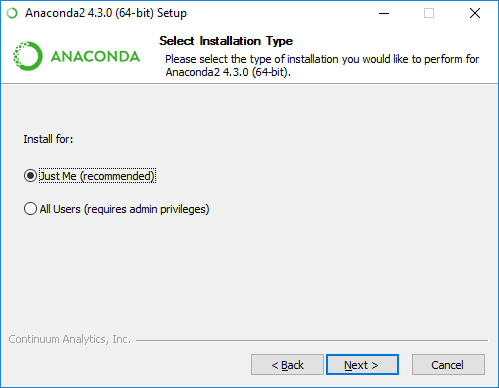Figure 1: Anaconda Navigator installation

Once Anaconda Navigator has been installed we need to create a new enviroment: Click on “Create” and type “Tableau-Python-Server” in the environment name, then click “Create”.

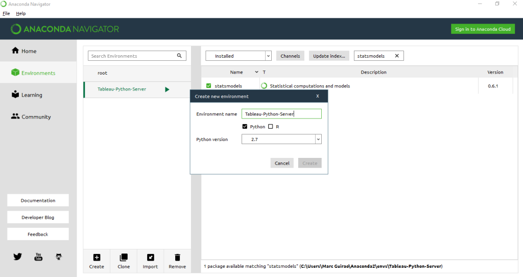Figure 2: Creating a new environment in Anaconda

This new environment will be used when connecting Tableau with TabPy. We also need some packages in order to perform mathematical calculations, apply machine learning algorithms, plot, define dataframes, create predictive models or edit Python code. We’re going to install the required packages: “Numpy”, “scikit-learn”, “matplotlib”, “pandas”, “statsmodel” and “ipython”; search for the packages in the “Not Installed” window and install them all.

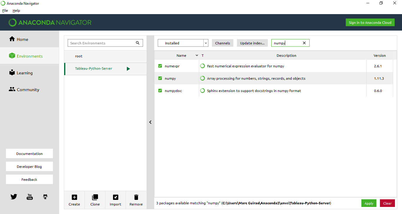Figure 3: Installing Python Packages

You can also download “Spyder”, a powerful Python IDE with advanced editing, interactive testing, debugging and introspection features, to try your Python code before using it in Tableau calculated fields. Go to the Home tab of Anaconda Navigator, and select the created environment “Tableau-Python-Server”; you can install “Spyder” from there.

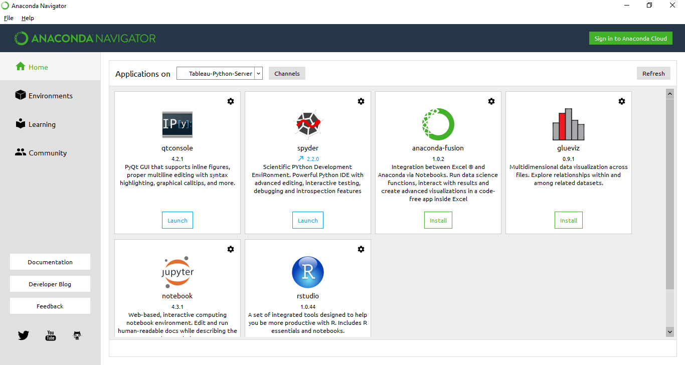Figure 4: Anaconda Navigator

2. Installing TabPy

Running Python code within a Tableau workbook requires a Python server to execute it, and the TabPy framework gets the job done. Download TabPy from github at the following link and decompress the file.

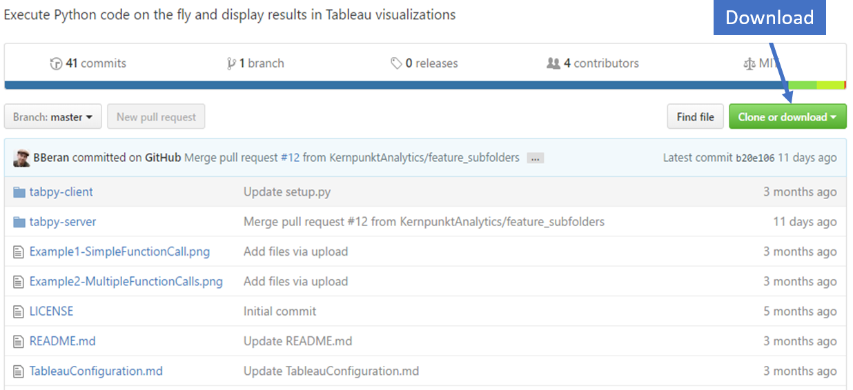Figure 5: Download Tabpy

On Windows prompt: activate Tableau-Python-Server In the TabPy folder run the following commands to install TabPy client and server as well as package dependencies.
pip install -r ./tabpy-server/requirements.txt pip install ./tabpy-client pip install ./tabpy-server As the packages are installed, you will see the install locations listed in the command line. These might look like /Users/username/anaconda/envs/Tableau-Python-Server/lib/python2.7/site-packages or \Users\username\anaconda\envs\Tableau-Python-Server\lib\site-packages depending on your environment. Navigate to the tabpy_server folder under site-packages and run startup.bat 9001. 9001 is the port to connect Tableau with the TabPy server.

3. Connecting Tableau with TabPy

The next step is to connect Tableau 10.2 with TabPy. This can be done in Help > Settings and Performance > Manage External Service Connection:

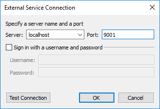Figure 6: Connecting Tableau + Python Server

Test the connection and you should get a “successfully connected” prompt. Now you can check out an example of predictive analysis.

4. Using Tableau + Python for predictive analytics

In this section, you can follow through an example of how to visualize a Time Series prediction with Tableau.

We’re going to use a dataset called AirPassengers, containing historic data on the number of passengers per month of an airline company. First, we open a new Tableau workbook and connect to the AirPassengers.csv dataset, then we create all calculated fields and parameters:

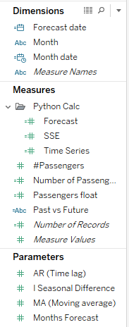Figure 7: Calculated fields and Dimensions

Define the parameters: We can create parameters to choose the number of autoregressive terms, the number of moving average terms and the seasonal differencing order to our arima time series model.

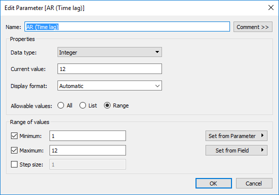Figure 8: Autoregresive terms

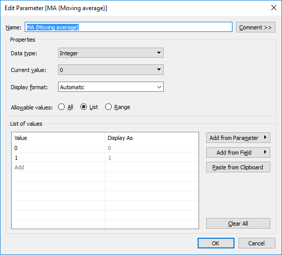Figure 9: Moving average terms

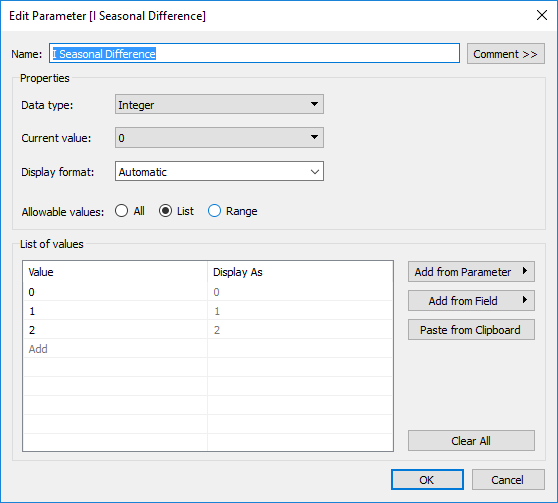Figure 10: Seasonal differencing order

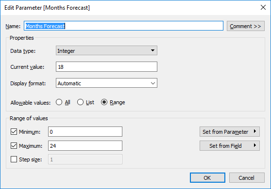Figure 11: Months to forecast

Time dimensions need to be formatted.

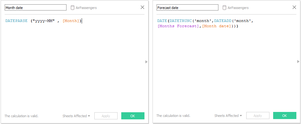Figures 12 and 13: Date parsing and Date shift

Finally we have to create the calculated fields. The measure “#Passengers” is defined as integer; we should fomat this field to assign float (number decimal) format, so we can combine axis of this measure with the predicted outcomes.

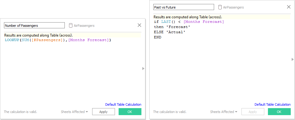Figures 14 and 15: Synchronize number of passengers with correspondent month and differentiate forecast values with predicted past values

Now we’re going to embed python code to the new calculated fields. The code embedded to the calculated field “Time Series” will return the predicted values of an Arima(p, d, q) model, where p=[AR (time lag)]; d=[I Seasonal Difference]; q=[MA (Moving Average)], with the parameters we created above. Find the python code below:

SCRIPT_REAL(
'
import pandas as pd
import numpy as np
import matplotlib.pylab as plt
from matplotlib.pylab import rcParams
dates = _arg1
passeng = _arg2
order_arima = min(_arg3)
seasonal_diff = min (_arg4)
ma_param = min (_arg5)
months_forecast = min(_arg6)
ts = pd.DataFrame({"dates": dates,"Passengers": passeng})
ts["Passengers"] = ts["Passengers"].astype("float64")
ts = ts.set_index(["dates"])
ts_log = np.log(ts)
ts_log.index = pd.to_datetime(ts_log.index)
ts_log_diff = ts_log - ts_log.shift()
ts_log_diff["Passengers"][0] = 0
from statsmodels.tsa.arima_model import ARIMA
model = ARIMA(ts_log_diff, order=(order_arima, seasonal_diff, ma_param))
results_ARIMA = model.fit(disp=-1)
predictions_value = results_ARIMA.forecast(months_forecast)[0]
from dateutil.relativedelta import relativedelta
add_month = relativedelta(months=1)
predictions_dates = list()
for i in range(months_forecast):
	predictions_dates.append ( results_ARIMA.fittedvalues.index[-1] + ((i+1)*add_month))
forecast_log_diff = pd.Series(predictions_value, index=predictions_dates)
predictions_ARIMA_diff = pd.Series(results_ARIMA.fittedvalues, copy=True)
predictions_ARIMA_diff_cumsum = predictions_ARIMA_diff.cumsum()
predictions_ARIMA_log = pd.Series(np.asscalar(ts_log.ix[0]), index=ts_log.index)
predictions_ARIMA_log = predictions_ARIMA_log.add(predictions_ARIMA_diff_cumsum,fill_value=0)
predictions_ARIMA = np.exp(predictions_ARIMA_log)
forecast_log_diff_ARIMA = pd.Series(forecast_log_diff, copy=True)
forecast_ARIMA_log_diff_cumsum = forecast_log_diff_ARIMA.cumsum()
forecast_ARIMA_log = pd.Series(np.asscalar(ts_log.ix[-1]), index=forecast_log_diff_ARIMA.index)
forecast_ARIMA_log = forecast_ARIMA_log.add(forecast_ARIMA_log_diff_cumsum,fill_value=0)
forecast_ARIMA = np.exp(forecast_ARIMA_log)
return list(predictions_ARIMA)
',
ATTR([Month]), ATTR([#Passengers]), MIN([AR (Time lag)]), MIN([I Seasonal Difference]), 
MIN([MA (Moving average)]), MIN([Months Forecast]))

For the forecasting part, create the calculated field “Forecast”:

SCRIPT_REAL(
'
import pandas as pd
import numpy as np
import matplotlib.pylab as plt
from matplotlib.pylab import rcParams
dates = _arg1
passeng = _arg2
order_arima = min(_arg3)
seasonal_diff = min (_arg4)
ma_param = min (_arg5)
months_forecast = min(_arg6)
ts = pd.DataFrame({"dates": dates,"Passengers": passeng})
ts["Passengers"] = ts["Passengers"].astype("float64")
ts = ts.set_index(["dates"])
ts_log = np.log(ts)
ts_log.index = pd.to_datetime(ts_log.index)
ts_log_diff = ts_log - ts_log.shift()
ts_log_diff["Passengers"][0] = 0
from statsmodels.tsa.arima_model import ARIMA
model = ARIMA(ts_log_diff, order=(order_arima, seasonal_diff, ma_param))
results_ARIMA = model.fit(disp=-1)
predictions_value = results_ARIMA.forecast(months_forecast)[0]
from dateutil.relativedelta import relativedelta
add_month = relativedelta(months=1)
predictions_dates = list()
for i in range(months_forecast):
	predictions_dates.append ( results_ARIMA.fittedvalues.index[-1] + ((i+1)*add_month))
forecast_log_diff = pd.Series(predictions_value, index=predictions_dates)
predictions_ARIMA_diff = pd.Series(results_ARIMA.fittedvalues, copy=True)
predictions_ARIMA_diff_cumsum = predictions_ARIMA_diff.cumsum()
predictions_ARIMA_log = pd.Series(np.asscalar(ts_log.ix[0]), index=ts_log.index)
predictions_ARIMA_log = predictions_ARIMA_log.add(predictions_ARIMA_diff_cumsum,fill_value=0)
predictions_ARIMA = np.exp(predictions_ARIMA_log)
forecast_log_diff_ARIMA = pd.Series(forecast_log_diff, copy=True)
forecast_ARIMA_log_diff_cumsum = forecast_log_diff_ARIMA.cumsum()
forecast_ARIMA_log = pd.Series(np.asscalar(ts_log.ix[-1]), index=forecast_log_diff_ARIMA.index)
forecast_ARIMA_log = forecast_ARIMA_log.add(forecast_ARIMA_log_diff_cumsum,fill_value=0)
forecast_ARIMA = np.exp(forecast_ARIMA_log)
forecast_ARIMA_2 = predictions_ARIMA.append(forecast_ARIMA)
forecast_ARIMA_2 = forecast_ARIMA_2[len(forecast_ARIMA):]
return list(forecast_ARIMA_2)
',
ATTR([Month]), ATTR([#Passengers]), min([AR (Time lag)]), MIN([I Seasonal Difference]),
MIN([MA (Moving average)]), MIN([Months Forecast]))

We have also included the sum of squared errors calculated field so that it is possible to compare different models. Here’s the code:

SCRIPT_REAL(
'
import pandas as pd
import numpy as np
import matplotlib.pylab as plt
from matplotlib.pylab import rcParams
dates = _arg1
passeng = _arg2
order_arima = min(_arg3)
seasonal_diff = min (_arg4)
ma_param = min (_arg5)
months_forecast = min(_arg6)
ts = pd.DataFrame({"dates": dates,"Passengers": passeng})
ts["Passengers"] = ts["Passengers"].astype("float64")
ts = ts.set_index(["dates"])
ts_log = np.log(ts)
ts_log.index = pd.to_datetime(ts_log.index)
ts_log_diff = ts_log - ts_log.shift()
ts_log_diff["Passengers"][0] = 0
from statsmodels.tsa.arima_model import ARIMA
model = ARIMA(ts_log_diff, order=(order_arima, seasonal_diff, ma_param))
results_ARIMA = model.fit(disp=-1)
predictions_value = results_ARIMA.forecast(months_forecast)[0]
from dateutil.relativedelta import relativedelta
add_month = relativedelta(months=1)
predictions_dates = list()
for i in range(months_forecast):
	predictions_dates.append ( results_ARIMA.fittedvalues.index[-1] + ((i+1)*add_month))
forecast_log_diff = pd.Series(predictions_value, index=predictions_dates)
predictions_ARIMA_diff = pd.Series(results_ARIMA.fittedvalues, copy=True)
predictions_ARIMA_diff_cumsum = predictions_ARIMA_diff.cumsum()
predictions_ARIMA_log = pd.Series(np.asscalar(ts_log.ix[0]), index=ts_log.index)
predictions_ARIMA_log = predictions_ARIMA_log.add(predictions_ARIMA_diff_cumsum,fill_value=0)
predictions_ARIMA = np.exp(predictions_ARIMA_log)
forecast_log_diff_ARIMA = pd.Series(forecast_log_diff, copy=True)
forecast_ARIMA_log_diff_cumsum = forecast_log_diff_ARIMA.cumsum()
forecast_ARIMA_log = pd.Series(np.asscalar(ts_log.ix[-1]), index=forecast_log_diff_ARIMA.index)
forecast_ARIMA_log = forecast_ARIMA_log.add(forecast_ARIMA_log_diff_cumsum,fill_value=0)
forecast_ARIMA = np.exp(forecast_ARIMA_log)
predictions_ARIMA_dataframe = pd.DataFrame(predictions_ARIMA)
SSE = sum((ts.ix[:,0]-predictions_ARIMA_dataframe.ix[:,0])**2)
return SSE
',
ATTR([Month]), ATTR([#Passengers]), MIN([AR (Time lag)]), MIN([I Seasonal Difference]),
MIN([MA (Moving average)]), MIN([Months Forecast]))

Finally, we’re going to design the view by dragging “Forecast date” (month level) to columns, “Number of Passengers” and “Forecast” to rows. Convert the plots to dual axis and then synchronize axis, obtaining this view:

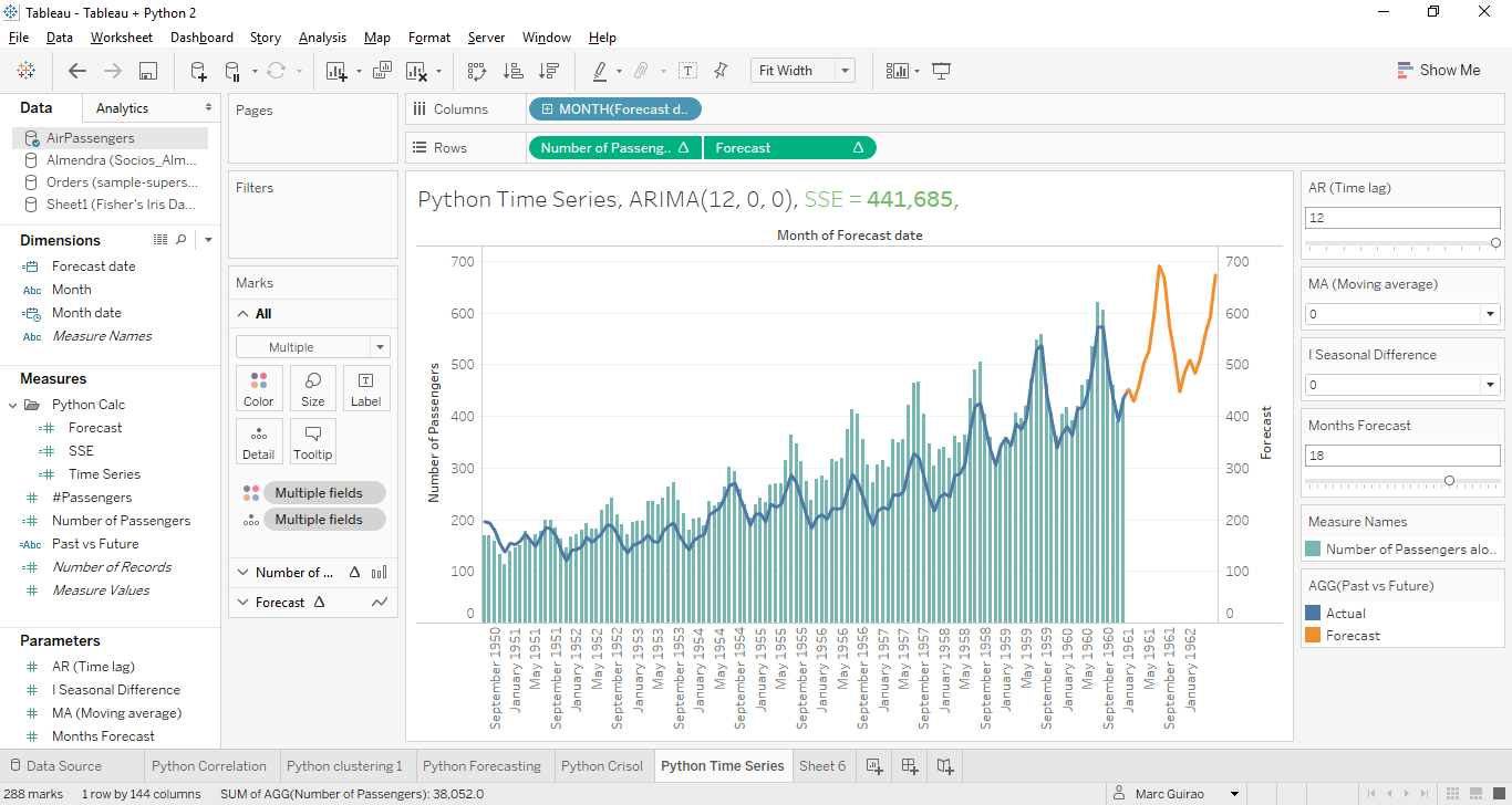Figure 16: Tableau + Python Predictive analysis view

Here you can see the real values as bars, predicted values as a blue line and forecast values as an orange line; you can play with different parameters to forecast more months or create a new ARIMA(p,d,q) model. Notice that the title is also dynamic – you can get this with:

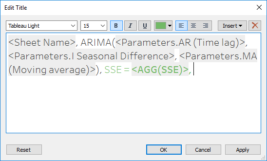Figure 17: Dynamic plot title

As you can see, it’s not the best model ever, so you can take it as a challenge to improve it!

Conclusion

To summarize, we have seen how to use Python code with Tableau, a new feature which gives us the opportunity to implement advanced analytics in our data. An example of Time Series prediction is included in this article. We can see a clear advantage to using this approach when compared to using the Tableau built-in tool set: adjustability of model parameters. We hope you enjoyed this article and please leave a comment if you have any doubts, suggestions or opinions. Stay tuned for future posts!

Click here if you would like to know more about the topic.

Tags:

Marc G

marc.guirao@clearpeaks.com