24 Apr 2025 Introduction to Vector Search in Oracle Database 23ai

The Oracle Database 23ai release introduces several exciting new features designed to enhance data management, app development, and workflow automation (you can find the complete list here). One of the most groundbreaking additions is Vector Search, which has the potential to transform the way we query and interpret data.

Instead of relying solely on keyword matching, Vector Search enables semantic understanding, allowing us to find job candidates, match products to users, or uncover insights based on meaning, context and relevance.

In this blog post we’ll take a closer look at this innovative feature, walk through a quick implementation guide, and share a practical use case to show how Vector Search can deliver real-world value.

Vector Search Overview

Vector Search introduces a new VECTOR data type, enabling the storage of data in vector format for semantic searches. Unlike traditional keyword-based queries, this feature uses VECTOR indexes to group similar data, improving search efficiency and enabling AI-powered operations directly within the database.

Here are some of this new feature’s key concepts:

• VECTOR Data Type: This can be used to store complex data like text or images as vectors (lists of numbers) in your database. You can specify parameters like the number of dimensions or the format when creating a vector column; you can find more information about the VECTOR data type here.
• VECTOR_DISTANCE Function: This function calculates how similar or different two vectors are, based on their distance calculated with a chosen metric, like Euclidean or cosine distance. It’s ideal for finding matches or comparing items, and you can discover more about the VECTOR_DISTANCE function here.
• VECTOR_EMBEDDING Function: This function transforms data into vectors using machine learning models, capturing essential features for advanced analysis or searches. You can learn more about the VECTOR_EMBEDDING function here.
• VECTOR Indexes: These are specialised indexes that group similar vectors to speed up similarity searches, enhancing performance when querying large datasets. You can find out more about vector indexes and how to create them here.

These tools simplify complex operations whilst maintaining the strong security and performance Oracle is known for. But how can they be used in an Oracle Database? Let’s have a quick look at how to implement and use this feature’s basic functionalities in Oracle Cloud Infrastructure (OCI).

Getting Started with Vector Search in an ADW

First of all, you’ll need to create a new Autonomous Database that uses the 23ai release. To do so, select Oracle Database and then Autonomous Database in the OCI main menu:

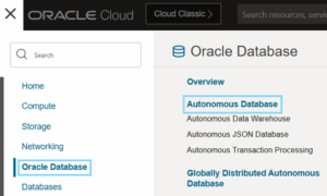
Figure 1. Accessing an Autonomous Database in OCI

There, select Create Autonomous Database and make sure to select 23ai as the version:

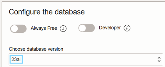
Figure 2. Choosing 23ai as the database version 

Once the database has been created, you can start using the new feature by clicking on SQL in the Database actions list:

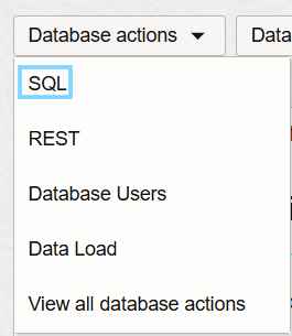
Figure 3. Accessing the SQL editor in the database

With the current settings both the VECTOR data type and the VECTOR_DISTANCE function are available for use, but you will need an embedding model in ONNX format if you want to use the VECTOR_EMBEDDING function.

To obtain a model in ONNX format, you can either convert a pretrained model (details on how to do so here) or download an existing one (the examples in this blog post use the all-MiniLM-L12-v2 model, but you could use other models such as GloVe or LaBSE).

To load the model, you will need to store it in an Object Storage Bucket and then access it from the database. However, you will only be able to access the Object Storage Bucket if you have a Credential, and to create one you will need an Auth token. Get one by clicking on Profile in the upper-right corner and selecting My Profile:

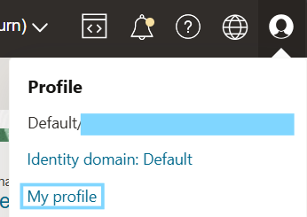
Figure 4. Accessing Profile to create an Auth token

Then, in the Resources menu in the lower-left corner, select Auth tokens:

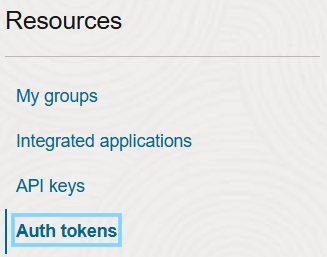
Figure 5. Selecting the Auth tokens option

Click on Generate token and enter a Description:

Figure 6. Generating Auth token

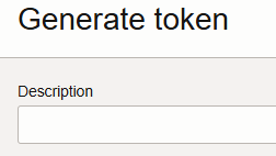
Figure 7. Generating Auth token

A token will be generated, which you can see and copy. Bear in mind that the token will not be shown again and you will need it later, so make sure you copy it now or you may have to create a new one later.

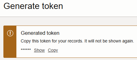
Figure 8. Auth token is generated

Now that you have your Auth token, you will need to create a Credential in the database, using the following code:

BEGIN 
    DBMS_CLOUD.CREATE_CREDENTIAL( 
    credential_name => '<CREDENTIAL_NAME>', 
    username => '<Your OCI username>', 
    password => '<Your Auth token>');  
END; 

After creating the Credential, you can use it to access the Object Storage Bucket and load the model using this query:

DECLARE  
    ONNX_MOD_FILE VARCHAR2(100) := '<model_name.onnx>'; 
    MODNAME VARCHAR2(500); 
    LOCATION_URI VARCHAR2(200) := '<Path to the Object Storage where the model is located>'; 
 
BEGIN 
    DBMS_OUTPUT.PUT_LINE('ONNX model file name in Object Storage is: '||ONNX_MOD_FILE);  
-------------------------------------------- 
-- Define a model name for the loaded model 
-------------------------------------------- 
    SELECT UPPER(REGEXP_SUBSTR(ONNX_MOD_FILE, '[^.]+')) INTO MODNAME from dual; 
    DBMS_OUTPUT.PUT_LINE('Model will be loaded and saved with name: '||MODNAME); 
 
----------------------------------------------------- 
-- Read the ONNX model file from Object Storage into  
-- the Autonomous Database data pump directory 
----------------------------------------------------- 
 
BEGIN DBMS_DATA_MINING.DROP_MODEL(model_name => MODNAME); 
EXCEPTION WHEN OTHERS THEN NULL; END; 
 
    DBMS_CLOUD.GET_OBJECT(                             
        credential_name => '<CREDENTIAL_NAME>', 
        directory_name => 'DATA_PUMP_DIR', 
        object_uri => LOCATION_URI||ONNX_MOD_FILE); 
 
----------------------------------------- 
-- Load the ONNX model to the database 
-----------------------------------------                    
 
    DBMS_VECTOR.LOAD_ONNX_MODEL( 
        directory => 'DATA_PUMP_DIR', 
        file_name => ONNX_MOD_FILE, 
        model_name => MODNAME); 
 
    DBMS_OUTPUT.PUT_LINE('New model successfully loaded with name: '||MODNAME); 
END; 

Once these steps have been completed, the model will be ready to use and you will be able to create vector embeddings. You can find more information on this process here.

Demo Use Case: Talent Acquisition

Now that everything’s set up, you can start experimenting with the primary functionalities of vectors and vector search. You can use your own datasets or even create entirely new ones in seconds using AI generative tools.

To showcase a specific use case that benefits from this feature, we have prepared a brief demo that covers all these functionalities in OCI, as well as presenting the results in a report in Oracle Analytics Cloud (OAC).

The chosen use case is talent acquisition. In this context, we will use two different tables, one with a series of available positions with details such as the job name, required skills, location, and years of experience needed, and another with a list of candidates looking for work, with information about their current roles, skills, location, and years of experience in that role.

As you may have guessed, the objective will be to convert this data into vectors and then compare them to find the most suitable candidate for each role based on the distance between them.

We’ll start by creating a table for each dataset. This can be done manually, or by using the Upload Data Into New Table option inside the Data Loading section of the Object submenu in the Navigator tab of the SQL editor:

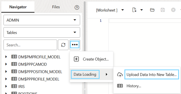
Figure 9. Loading data into the database

There, we can visualise and configure how the data will be inserted in the table:

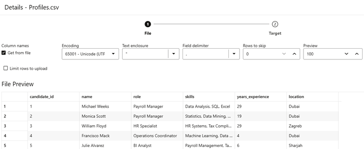
Figure 10. Data Load Configuration

Now that both tables are ready (let’s call them PROFILES and POSITIONS), we can start using the new features, first creating new columns to store the vectors that we will generate:

ALTER TABLE USER23AI.PROFILES ADD VECTOR_COLUMN_NAME VECTOR;

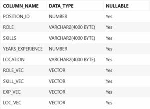
Figure 11. Vector columns created

The next step is to generate the vector for each desired column, using the VECTOR_EMBEDDING function and the loaded embedding model:

SELECT 
    ROLE,
    VECTOR_EMBEDDING(ALL_MINILM_L12_V2 USING ROLE AS DATA) AS ROLE_VEC 
FROM USER23AI.PROFILES
WHERE ROWNUM < 5;

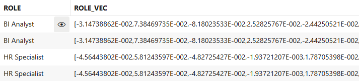
Figure 12. Overview of generated vectors for Role column

Now that all the vectors have been generated, we can start to compare distances between columns from both tables using the VECTOR_DISTANCE function:

select 
    pos.position_id, 
    pos.role as pos_role, 
    prof.role as prof_role, 
    vector_distance(pos.role_vec, prof.role_vec, cosine) as dist 
from 
    USER23AI.profiles prof, 
    USER23AI.positions pos
order by pos.position_id;

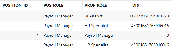
Figure 13. Distance between Role vectors

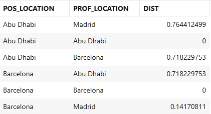
Figure 14. Distance between Location vectors

With this data, we can take it a step further by ranking the rows based on the vector distance for the relevant columns, retaining only the top-ranked row (i.e. the one with a distance closest to or equal to 0). This way, we obtain the candidate whose profile is the most similar to the position offered:

WITH RankedProfiles AS (
    SELECT 
        pos.POSITION_ID, 
        pos.ROLE AS OFFERED_ROLE, 
        pos.SKILLS AS DESIRED_SKILLS, 
        pos.YEARS_EXPERIENCE AS DESIRED_YEARS_OF_EXPERIENCE,
        pos.LOCATION AS POSITION_LOCATION,
        prof.NAME AS CANDIDATE_NAME,
        prof.ROLE AS CURRENT_ROLE, 
        prof.SKILLS AS SKILLS, 
        prof.YEARS_EXPERIENCE AS YEARS_OF_EXPERIENCE,
        prof.LOCATION AS LOCATION,
        -- Rank candidates for each position based on cosine similarity
        ROW_NUMBER() OVER (
            PARTITION BY pos.POSITION_ID 
            ORDER BY 
                VECTOR_DISTANCE(prof.ROLE_VEC, pos.ROLE_VEC, COSINE),
                VECTOR_DISTANCE(prof.SKILL_VEC, pos.SKILL_VEC, COSINE),
                VECTOR_DISTANCE(prof.LOC_VEC, pos.LOC_VEC, COSINE),
                VECTOR_DISTANCE(prof.EXP_VEC, pos.EXP_VEC, COSINE)
        ) AS rank
    FROM 
        USER23AI.PROFILES prof, 
        USER23AI.POSITIONS pos
)
-- Retrieve only the top-ranked profile for each position
SELECT 
    POSITION_ID, 
    OFFERED_ROLE, 
    DESIRED_SKILLS, 
    DESIRED_YEARS_OF_EXPERIENCE,
    POSITION_LOCATION,
    CANDIDATE_NAME,
    CURRENT_ROLE, 
    SKILLS, 
    YEARS_OF_EXPERIENCE,
    LOCATION
FROM RankedProfiles
WHERE rank = 1
ORDER BY POSITION_ID;

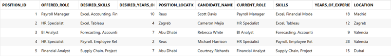
Figure 15. Most suitable candidate for each position

Now we can try some different approaches to the search configurations to get slightly different results:

• Modifying the order of execution for the vector searches will change the results, giving more weight to the earlier searches.
• Using the sum of all search results as a single ordering component will also change the results.
• Using the last approach as a base, we can assign different weights to the components of the sum to further tailor the results.

As you can see, it’s not particularly difficult to perform vector-related operations in the database, but what if we want to create a report with this data? Well, vector operations are not directly available in OAC, but there are some workarounds that will let us show the results and even change some parameters.

First, we’ll need to create a connection to the database and then generate a dataset. For this example, we created a dataset that combines all the data from the POSITIONS and PROFILES tables. We included vector columns for all relevant fields in these tables, though the distance values were not stored. So, how can we calculate them in OAC?

One simple solution would be to add new columns to the database to store these values, but we opted for a different approach. By using the EVALUATE function, we can execute SQL functions that are not directly supported in OAC, using report columns as input parameters.

We’ll use this function to calculate the distances. What’s more, by creating a parameter that lists all possible search metrics, we can choose the metric in the report by including a CASE structure in the calculation, running this code:

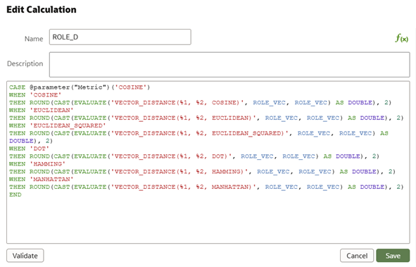
Figure 16. Vector distance calculation using the EVALUATE function

Now we can create an additional calculated field to aggregate the weighted distances across the relevant column. This field will allow us to rank the results by position ID and display a number of top matches corresponding to the number of candidates selected:

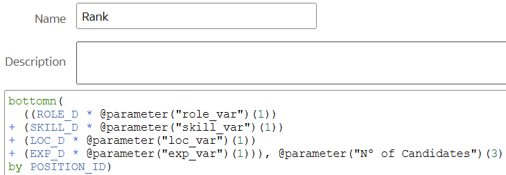
Figure 17. Final overview of the report

This approach produces a report that not only identifies the most suitable candidates for each position but also allows us to modify the search metric, adjust the weighting of each column, and control the number of candidates displayed:

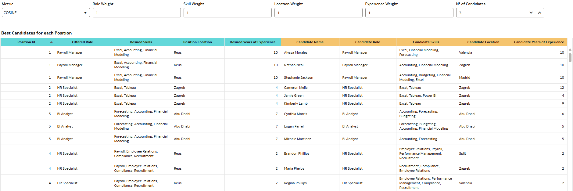
Figure 18. Final overview of the report

Now, imagine the following situation: we want to focus on identifying candidates whose skill sets closely match the requirements of the position, regardless of their current role or professional experience; location is less of a concern, as the position is fully remote. By adjusting the weighting of each parameter used in the search, we can tailor the results accordingly and get a different set of candidate matches:

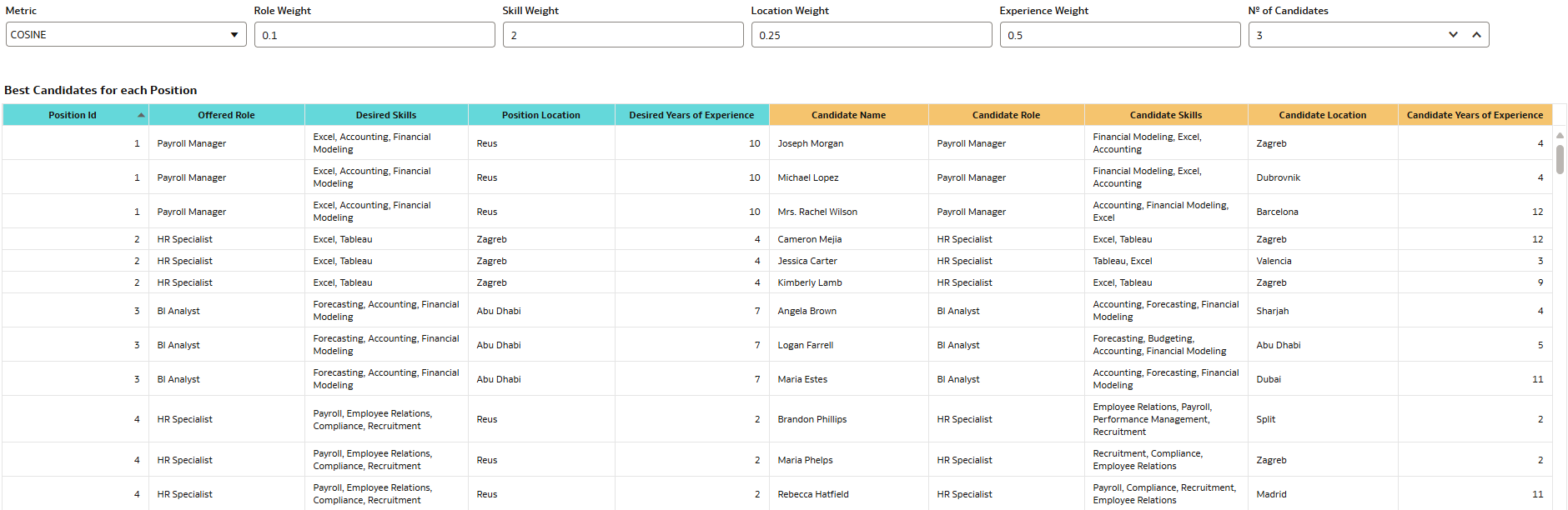
Figure 19. Results after changing parameter weights

Changing the search metric can also affect the results, as you can see below:

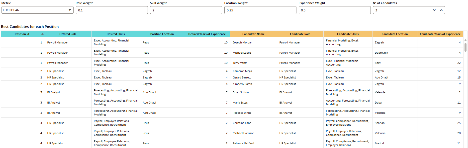
Figure 20. Results after changing search metric

Conclusions

The Vector Search feature in Oracle Database 23ai enables semantic search capabilities, opening up a wide range of possibilities for data analysis and application development. Combined with its flexibility in managing diverse data types and its compatibility with pretrained models, this functionality represents a powerful asset for AI-driven operations and supports a virtually limitless range of use cases across various industries.

The only limitation is the absence of native support in OAC. However, future updates are expected to address this. In the meantime, workarounds, like the one demonstrated in this blog post, allow us to use these capabilities within the platform to some extent.

Interested in exploring how Vector Search and AI capabilities can drive innovation in your business? Reach out to us today! Our certified experts are ready to help you harness the full potential of your Oracle tech stack.