22 May 2024 How to Display a Dynamic Column in Power BI Based on Viewer Profile
Requests to implement Row Level Security (RLS) in Power BI dashboards are on the rise as the application consolidates its position as a favourite reporting tool.
Most dashboards are designed for a very specific audience, but what if they need to cater to a broader group with varying requirements for data granularity? Or what if different data needs to be displayed based on RLS in a particular visual?
In this blog post, we are going to present a standard solution to the challenges outlined above. Our goal is to modify data granularity visualisation in a bar chart by changing the X-axis data according to the organisation level to which the user belongs.
Solution
Initial Requirements:
- Display the project stage for each company division and department using a bar chart.
- A user can only view their own projects, or those associated with their lower organisation hierarchy.
- The data should be visualised according to the user’s hierarchy, with the option to drill down for more granularity if a lower organisation level is available.
We’ll use the following hierarchy:
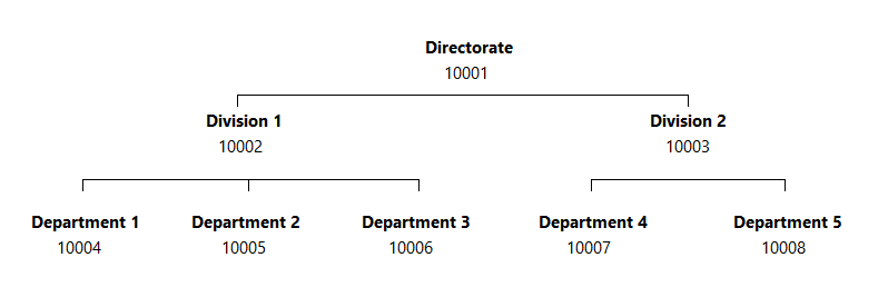
Figure 1: Organisation Level
The sample data used for this representation is composed of:
- Employee Table (D): Organisation employee data.
- Projects Table (F): Project-related data, like name, stage, or status.
It is important to note that the Employee Manager Key Path (EMP_PATH_TX) must be imported into the Projects Table. This is because RLS will filter data for a single user only, and as stated in the second point of the Initial Requirements, we also aim to capture projects managed by other users that belong to lower levels.
To assign the necessary organisation level to each user, we have added a calculated column named ORG_LEVEL_TX, with this logic:
IF (ORG_LEVEL1_TX = ORG_LEVEL2_TX, ORG_LEVEL2_TX, ORG_LEVEL3_TX)
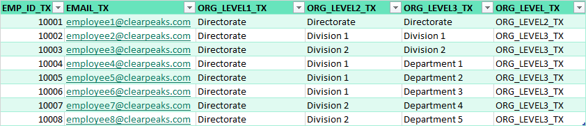
Figure 2: Employee Table
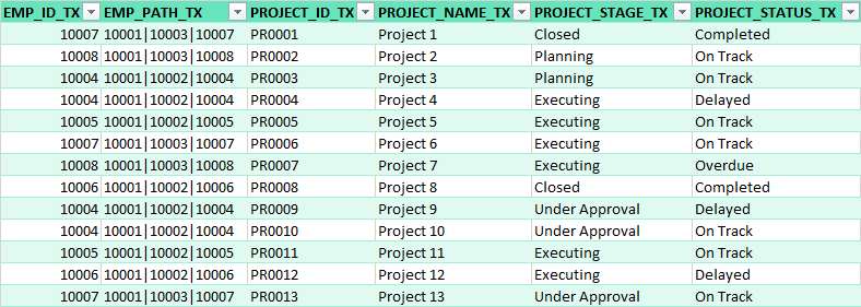
Figure 3: Projects Table
Once these tables have been imported into the Power BI model, we have to create a calculated table, named Parameter, to define the columns that we want to switch based on the RLS settings; this will be used as the X-axis in our visualisations.
As outlined below, three fields are necessary within the function to define this table:
- Column Name: the first field specifies the name the column will take visually. For initial testing to ensure the visual changes accordingly, we will keep the Employee Table nomenclature and only change the names for columns that will be repeated in drilldowns.
- Data Source: the second field is the physical column from which we want to extract data, utilising the NAMEOF() function.
- Index Number: the third field is an index number, used to add additional columns that act as drilldown levels, facilitating a deeper data analysis.
Parameter (Calculated Table)
Parameter = {
    ("ORG_LEVEL2_TX", NAMEOF('Employee'[ORG_LEVEL2_TX]), 0),
    ("Department [Directorate Level]", NAMEOF('Employee'[ORG_LEVEL3_TX]), 0),
    ("ORG_LEVEL3_TX", NAMEOF('Employee'[ORG_LEVEL3_TX]), 1)
}
The last table to be defined is the Bridge Table, which will serve as the link between the Parameter and Employee Tables. This is necessary because a many-to-one relationship is not allowed when the join column is used as the primary key.
All column names specified in the Parameter Table will populate the Join Parameter column, and the organisation level to which the respective column name correlates will populate the Join Employee column:
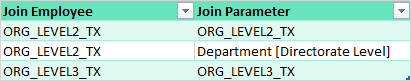
Figure 4: Bridge Table
Now that all the tables are in the model, let’s join them. As all the logic is based on employee data, the Employee Table filters the Projects Table, which acts as the fact table, based on EMP_ID_TX. At the same time, the Employee Table applies a filter to the Bridge Table on ORG_LEVEL_NUM = Join Employee. Finally, the Bridge and Parameter Tables are filtered in both directions on Join Parameter = Parameter:
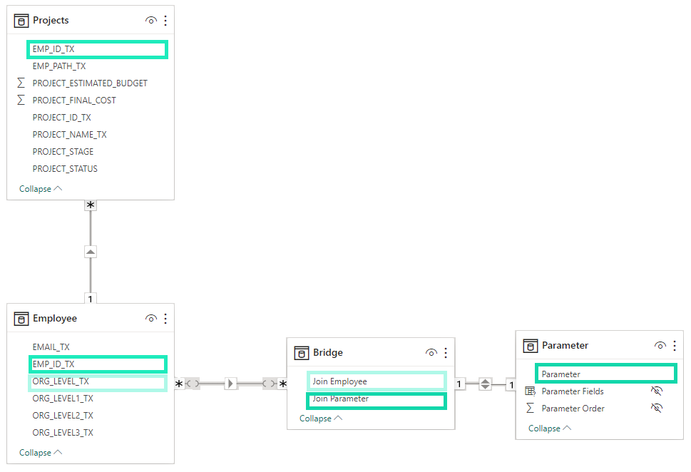
Figure 5: Power BI Model
RLS will be configured in both the Bridge and Projects Tables. In the Bridge Table, we will get the organisation level from the user accessing the system, which leads to filtering the Parameter Table:
CONTAINSTRING([Join Employee], LOOKUPVALUE('Employee'[ORG_LEVEL_TX], 'Employee'[EMAIL_TX], UPPER(userprincipalname())))
For the Projects Table we will filter each project where the user is part of the organisation hierarchy path:
CONTAINSTRING([EMP_PATH_TX], LOOKUPVALUE('Employee'[EMP_ID_TX], 'Employee'[EMAIL_TX], UPPER(userprincipalname())))
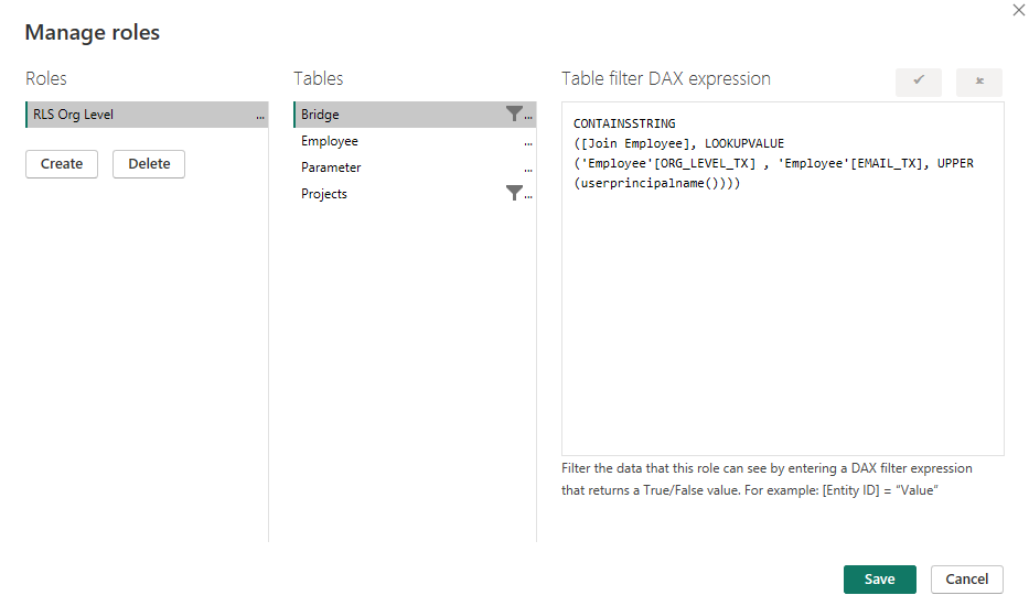
Figure 6: Security Bridge Table
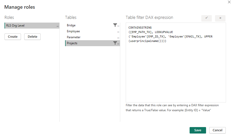
Figure 7: Security Projects Table
The last step is to add data to the visual, which in this case will be a stacked column chart:
• X-axis: ‘Parameter’ [Parameter].
• Y-axis: Count of ‘Projects’ [PROJECT_ID_TX] as # Projects.
• Legend: ‘Projects’ [PROJECT_STAGE] as Stage.
Result
If Employee 1 is accessing the data, who according to the Employee Table should see ORG_LEVEL2_TX, the first organisation level in the bar chart X-axis is Division. Since Employee 1 is part of both Divisions, all data is available. Note that the drill-down feature is enabled and will show all the departments to which the user belongs in the X-axis:
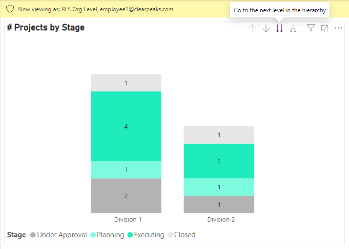
Figure 8: First level view as User: Employee 1
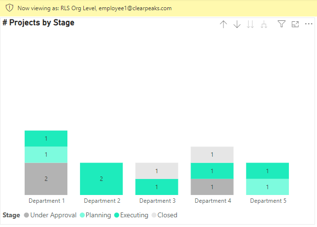
Figure 9: Second level view as User: Employee 1
If Employee 2 or Employee 3 access the data, they should, according to the Employee Table, view ORG_LEVEL3_TX. Department will be the default view. Figures 10 and 11 illustrate that Departments 1, 2, and 3 are accessible to Employee 2, while Departments 4 and 5 are available to Employee 3:
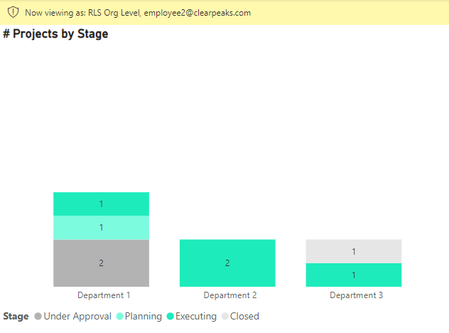
Figure 10: Level view as User: Employee 2
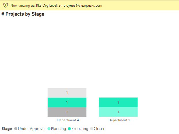
Figure 11: Level view as User: Employee 3
If the user is Employee 7, who should see ORG_LEVEL3_TX, Department will be the default view as in the previous example, but in this case only Department 4 will be visible:
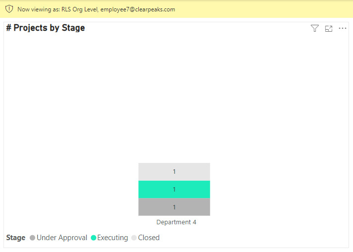
Figure 12: Level view as User: Employee 7
Conclusion
This configuration facilitates the reuse of a single visualisation for diverse purposes in Power BI. Although in this instance we opted to modify only one axis, based on the organisation level of the user accessing the data, we could also alter the dimension displayed, where ‘dimension’ refers to a column in a dataset. The ability to present different granularities and dimensions within the same visual simplifies contextual understanding, as each user views data that is familiar to them.
For additional clarification or support, please don’t hesitate to contact our consultants here at ClearPeaks. Our experts are dedicated to helping you harness the full potential of your data visualisation tools, ensuring optimal results.