19 Mar 2025 Operationalising ML with Snowflake and Fabric Integration – Part 2

In this continuation of our ETL pipeline project, we’re enhancing the architecture established in Part 1 by adding data ingestion through Azure Blob Storage, using the compute power of Snowpark and Snowflake ML models, as well as integrating with Microsoft Fabric and Power BI for reporting and visualisation. First, let’s recap the technologies we presented in our previous blog article.

Initial ETL Setup:

1. dbt for transformations: dbt organises and runs data transformations in Snowflake, structuring raw data into refined, analysis-ready tables.
2. Snowflake as the data warehouse: Snowflake serves as our central data storage, where dbt transformations are executed on large datasets.
3. Airflow for orchestration: Airflow automates the ETL process, using DAGs to manage and sequence dbt jobs, enabling regular updates and pipeline monitoring.

With this base in place, we can add more advanced features, such as ML models orchestrated with Airflow. This setup allows us to track data from its raw state through to the final analysis, enabling us to predict whether a user is likely to leave the telecom company (based on a fictional dataset).

For a more in-depth setup and a deeper exploration of using models with Snowpark, take a look at the following articles on creating a Data Science environment with Anaconda:

• Using Snowpark and Model Registry for Machine Learning – Part 1
• Using Snowpark and Model Registry for Machine Learning – Part 2

And if you want to learn even more about advanced models, you can refer to this mini-series:

• LLMs in Snowflake: Discovering Cortex Functions – Part 1
• LLMS in Snowflake: Discovering Cortex Functions – Part 2

Data Flow

The data pipeline for this PoC starts with raw data stored in Microsoft Azure, which is processed and orchestrated by Apache Airflow, then transferred to Snowflake for further analysis with Snowpark’s compute power. From Snowflake, the data is mirrored to Microsoft Fabric to create a synchronised copy. Finally, Power BI connects using a Direct Lake connection to generate reports.

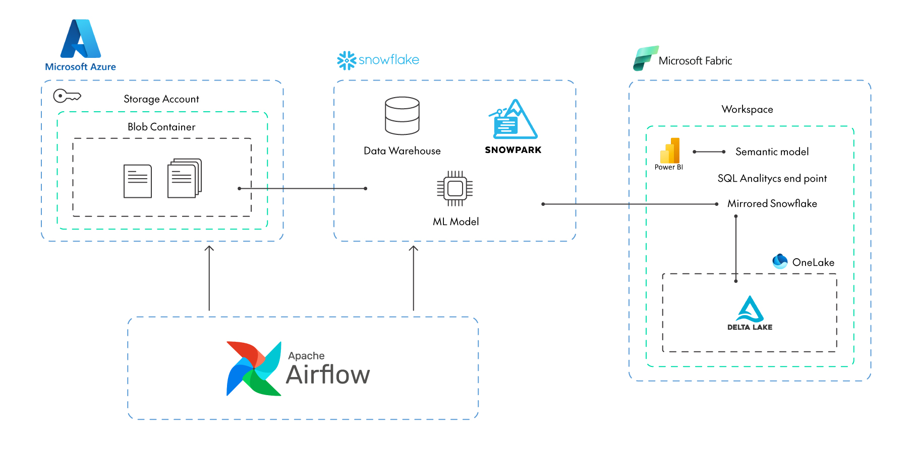
Figure 1: Architecture

Move Data from Azure Blob Storage to Snowflake

Azure Blob Storage provides a secure and scalable storage area for raw data files before they are ingested into a data warehouse like Snowflake for further processing and analysis.

To manage and automate these data flows, we’ll use Airflow. This orchestration tool allows us to schedule, monitor and log every step of the data pipeline, ensuring full visibility into the progress and status of data loads.

Let’s get to work! The first thing to do is to update the project requirements.txt file by adding the azure-storage-blob dependency:

azure-storage-blob==12.19.0

As we saw in our first blog post, remember to define the connections in Airflow’s Connections section to ensure smooth integration and secure credential management.

Once we have defined the account_url, credential and container_name parameters, we can write a function to connect to Azure Blob Storage. As we can see, the get_blob_files function connects to an Azure Blob Storage account and retrieves a list of file names from a specific container. The transfer_blob_to_snowflake function downloads each file from the Azure container to a temporary local file, and then a Snowflake PUT command is used to upload it to a specific location (stage) within Snowflake:

AZURE_CONN_ID = 'azure-blob-storage-conn'
SNOWFLAKE_CONN_ID = 'snowflake_conn'
SNOWFLAKE_STAGE = '@MY_INT_STAGE'

def get_blob_files(**kwargs):
    wasb_hook = WasbHook(wasb_conn_id=AZURE_CONN_ID)
    azure_conn = wasb_hook.get_conn()
    extras = azure_conn.extra_dejson
    
    account_url = extras.get("account_url")
    credential = extras.get("credential")
    container_name = extras.get("container_name")
    
    blob_service_client = BlobServiceClient(account_url=account_url, credential=credential)
    container_client = blob_service_client.get_container_client(container_name)

    blobs = container_client.list_blobs()
    blob_files = [blob.name for blob in blobs]
    
    return blob_files

def transfer_blob_to_snowflake(**kwargs):
    wasb_hook = WasbHook(wasb_conn_id=AZURE_CONN_ID)
    snowflake_hook = SnowflakeHook(snowflake_conn_id=SNOWFLAKE_CONN_ID)
    
    azure_conn = wasb_hook.get_conn()
    extras = azure_conn.extra_dejson
    account_url = extras.get("account_url")
    credential = extras.get("credential")
    container_name = extras.get("container_name")
    
    blob_files = get_blob_files(**kwargs)
    
    blob_service_client = BlobServiceClient(account_url=account_url, credential=credential)

    for blob_name in blob_files:
        try:
            blob_client = blob_service_client.get_blob_client(
                container=container_name, 
                blob=blob_name
            )

            with tempfile.NamedTemporaryFile(delete=False) as temp_file:
                blob_content = blob_client.download_blob().readall()
                temp_file.write(blob_content)
                temp_file_path = temp_file.name
    
            with snowflake_hook.get_conn() as conn:
                with conn.cursor() as cursor:        
                    stage_file_path = f"@{SNOWFLAKE_STAGE}/{blob_name}"
                    put_command = (
                        f"PUT 'file://{temp_file_path}' '{stage_file_path}' "
                        "AUTO_COMPRESS=TRUE OVERWRITE=TRUE"
                    )
                    cursor.execute(put_command)

        except Exception as e:
            print(f"Error processing file {blob_name}: {str(e)}")
            raise

Creating a Simple ML Model with Snowpark

In this section, we’ll demonstrate how Snowpark can help us to build a predictive model to identify users likely to unsubscribe from a fictitious telecom company. Using data stored in Snowflake, we’ll employ two popular machine learning algorithms, XGBoost and Random Forest, to build this model.

Snowpark lets us process our telecom dataset quickly, train our models, and generate predictions, all within the Snowflake ecosystem. This approach not only simplifies the workflow but also allows large-scale data processing without the need for external resources.

The first step in building our ML model is to import the necessary dependencies, just as we did in the previous section:

snowflake-connector-python==3.12.2
snowflake-snowpark-python==1.22.1
snowflake-ml-python==1.6.4

Once we’ve installed the libraries, we need to create a method to set up a Snowpark session:

def create_snowpark_session():
    conn = BaseHook.get_connection('snowflake_conn')
    
    snowpark_config = {
        'user': conn.login,
        'password': conn.password,
        'account': conn.extra_dejson.get('account'),
        'warehouse': conn.extra_dejson.get('warehouse'),
        'database': conn.extra_dejson.get('database'),
        'schema': conn.extra_dejson.get('schema'),
        'role': conn.extra_dejson.get('role')
    }
    
    return Session.builder.configs(snowpark_config).create()

We start the training by connecting to Snowpark and retrieving the Gold ML_DATASET layer, preprocessed for machine learning analysis.

With Snowpark, data is loaded from Snowflake directly, where queries are executed, and results are handled in Snowpark as distributed data structures. This approach optimises performance, reducing data transfer by processing in the Snowflake warehouse:

def snowpark_ml(**kwargs):
    session = create_snowpark_session()
    data = session.sql("select * from POC_DBT_AIRFLOW.GOLD.ML_DATASET")

Once the data has been loaded, we split it randomly into training and testing datasets. The training set will be used to train the machine learning models, whilst the test set will be used to evaluate them:

train_data, test_data = data.random_split(weights=[0.8, 0.2], seed=0)

In our example, we’re using a set of features (customer details) to predict the target variable, which is the CUSTOMER_STATUS; we’ve excluded CUSTOMER_ID as it doesn’t contribute to the predictions. We won’t go into more details about feature engineering here, as it’s not the purpose of this article, but we must analyse the data thoroughly to determine which elements can help us (and which ones can’t) in creating predictive models:

feature_cols = train_data.columns
feature_cols.remove('CUSTOMER_STATUS')
feature_cols.remove('CUSTOMER_ID')
target_col = ['CUSTOMER_STATUS']
output_colss = ['PREDICTION']

We’re training two machine learning models, XGBoost and Random Forest, both available in the Snowflake ML library.

The XGBoost model is a powerful gradient-boosting algorithm, widely used for classification tasks due to its accuracy and efficiency in handling complex data patterns:

XGBCmodel = XGBClassifier(
            input_cols=feature_cols, 
            label_cols=target_col, 
            output_cols=output_colss,
            enable_snowflake_compute=True
        )
        XGBCmodel.fit(train_data)
        XGBCmodel_predict = XGBCmodel.predict(test_data)

Random Forest is another common classification model that builds multiple decision trees and combines their predictions:

RandomForestmodel = RandomForestClassifier(
            input_cols=feature_cols, 
            label_cols=target_col, 
            output_cols=output_colss,
            enable_snowflake_compute=True
        )
        RandomForestmodel.fit(train_data)
        RandomForest_predict = RandomForestmodel.predict(test_data)

After training the models, we’ll evaluate their performance using standard classification metrics such as accuracy, precision, recall, and F1-score. These metrics help to determine how well each model identifies users who are likely to unsubscribe:

XGBoost Evaluation

# XGBoost Evaluation
XGBC_eval_accuracy = accuracy_score(df=XGBCmodel_predict, y_true_col_names='CUSTOMER_STATUS', y_pred_col_names='PREDICTION')
XGBC_eval_precision = precision_score(df=XGBCmodel_predict, y_true_col_names='CUSTOMER_STATUS', y_pred_col_names='PREDICTION')
XGBC_eval_recall = recall_score(df=XGBCmodel_predict, y_true_col_names='CUSTOMER_STATUS', y_pred_col_names='PREDICTION')
XGBC_eval_f1 = f1_score(df=XGBCmodel_predict, y_true_col_names='CUSTOMER_STATUS', y_pred_col_names='PREDICTION')

Random Forest Evaluation

# Random Forest Evaluation
RandomForest_eval_accuracy = accuracy_score(df=RandomForest_predict, y_true_col_names='CUSTOMER_STATUS', y_pred_col_names='PREDICTION')
RandomForest_eval_precision = precision_score(df=RandomForest_predict, y_true_col_names='CUSTOMER_STATUS', y_pred_col_names='PREDICTION')
RandomForest_eval_recall = recall_score(df=RandomForest_predict, y_true_col_names='CUSTOMER_STATUS', y_pred_col_names='PREDICTION')
RandomForest_eval_f1 = f1_score(df=RandomForest_predict, y_true_col_names='CUSTOMER_STATUS', y_pred_col_names='PREDICTION')

We’ll return the evaluation metrics and predictions to Snowflake after assessing the models. This makes it simpler to examine the predictions and to monitor their performance over time:

metrics = {
            'Model': ['XGBC']*4 + ['RandomForest']*4,
            'Measure': ['Accuracy', 'Precision', 'Recall', 'F1']*2,
            'Result': [
                XGBC_metrics['accuracy'], XGBC_metrics['precision'], 
                XGBC_metrics['recall'], XGBC_metrics['f1'],
                RF_metrics['accuracy'], RF_metrics['precision'], 
                RF_metrics['recall'], RF_metrics['f1']
            ]
        }
        metrics_df = pd.DataFrame(metrics)

Now it’s time to write the predictions into the Snowflake ML_PREDICTION table:

# Write predictions to Snowflake
RandomForest_predict.write.save_as_table("ML_PREDICTION", mode="overwrite")
session.create_dataframe(metrics_df).write.save_as_table("ML_SCORES", mode="overwrite")

session.close()

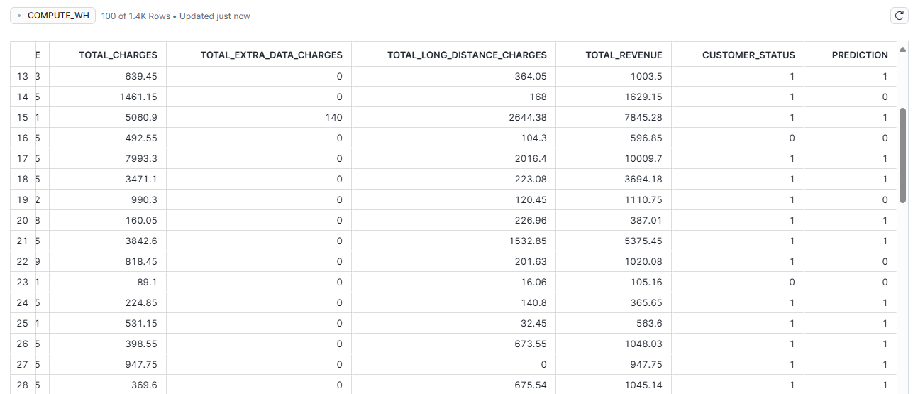
Figure 2: ML_PREDICTION table in Snowflake

Finally, we’ll save the training session metrics, which will facilitate the tracking of the model’s performance over time, and the analysis of the predictions:

# Write evaluation metrics to Snowflake
metrics_df = session.write_pandas(metrics_df, "ML_SCORES", auto_create_table=False, overwrite=True)

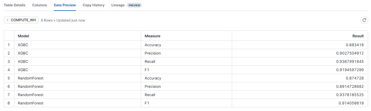
Figure 3: ML_SCORES table in Snowflake

To finalise the process, deploy the model and save it in the Snowflake registry, enabling easy reuse without the need to reload it every time. Once registered, the model can be imported and used for predictions whenever the data matches its specifications. A step-by-step guide, along with the necessary configurations, can be found in our blog post “Using Snowpark and Model Registry for Machine Learning – Part 2”, specifically in the section “Using Model Registry to Deploy ML Models.”

Upgrading Airflow DAG

Once the functions for retrieving data from Azure Blob Storage have been completed (transfer_blob_to_snowflake and snowpark_ml) and the ML model has been created, the next step is to modify our existing Airflow DAG to include these functions. The result is a structured pipeline where tasks run sequentially: transfer_task >> dbt_tg >> ml >> e2. This workflow covers data transfer, dbt transformations, machine learning, and a final task to mark completion. This setup ensures an end-to-end, orchestrated pipeline managed entirely by Airflow:

with DAG(
    dag_id="poc_dbt_snowflake",
    start_date=datetime(2024, 10, 30),
    schedule_interval=None,
):

    transfer_task = PythonOperator(
        task_id='transfer_task',
        provide_context=True,
        python_callable=transfer_blob_to_snowflake
    )

    dbt_tg = DbtTaskGroup(
        project_config=ProjectConfig("/usr/local/airflow/dags/dbt/dbtproject"),
        operator_args={"install_deps": True},
        execution_config=ExecutionConfig(dbt_executable_path=f"{os.environ['AIRFLOW_HOME']}/dbt_venv/bin/dbt",),
        profile_config=profile_config
    )

    ml = PythonOperator(
        task_id='machinelearning_model',
         provide_context=True,
        python_callable=snowpark_ml
    )

    e2 = EmptyOperator(task_id="post_dbt_and_ml")

    transfer_task >> dbt_tg >> ml >> e2

The final DAG is structured as shown below, with the dbt_task_group section in the middle. This component was covered in detail in the first part of this blog series:

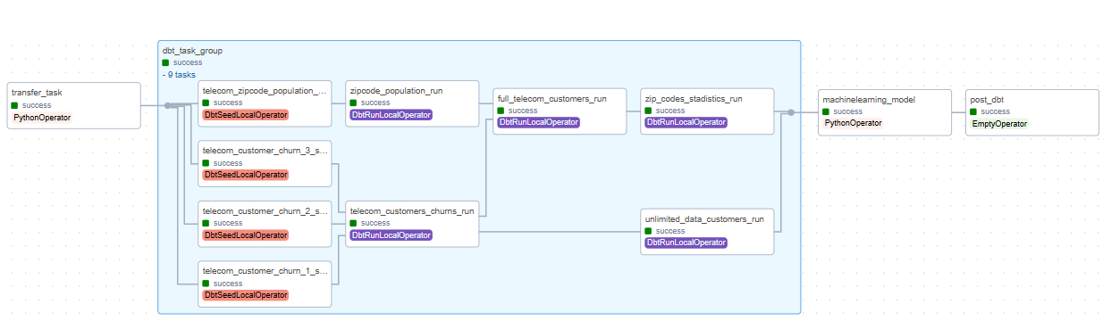
Figure 4: DAG Airflow

Connecting Snowflake to Microsoft Fabric with the Mirrored Option

With its Mirroring feature, Microsoft Fabric now offers a simplified way to integrate Snowflake warehouse data, enabling seamless data replication from Snowflake straight into Fabric’s OneLake environment, eliminating intricate ETL processes:

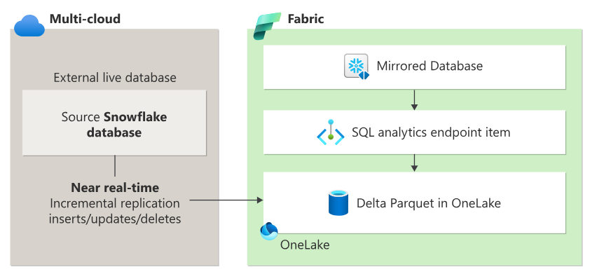
Figure 5: Architecture – Mirrored Snowflake

Key Benefits

Fabric Mirroring has a significant advantage as it provides a unified approach to data management, removing the need to handle services from multiple providers. This end-to-end integrated solution simplifies analytical workflows, facilitates collaboration between Microsoft and Snowflake, and ensures compatibility with thousands of solutions through the open-source Delta Lake table format.

Core Components

When you set up Mirroring in your Fabric workspace, three essential components are created:

• Mirrored database: Manages data replication to OneLake, converting it to Parquet for advanced analytics scenarios.
• SQL analytics endpoint: Provides read-only access to the mirrored data.
• Default semantic model: Powers business intelligence capabilities.

Limitations

• Table Limit Restriction: There’s a strict limit of 500 tables per database.
• Network Infrastructure Limitation: Snowflake instances behind virtual or private networks are not compatible with Fabric Mirroring.
• Authentication Restriction: Only basic username/password authentication is supported for Snowflake.

How to Implement Mirroring

First, we click on New Item and select the Mirrored Snowflake option:

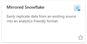
Figure 6: Mirrored Snowflake Option

Next, we configure the Snowflake connection using the URL and log in with a username and password:

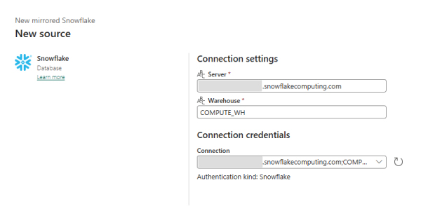
Figure 7: Connection Settings

Now we select the POC_DBT_AIRFLOW database and choose the tables we want to mirror. In our case we will use the previously created ML_Prediction and ML_Scores tables:

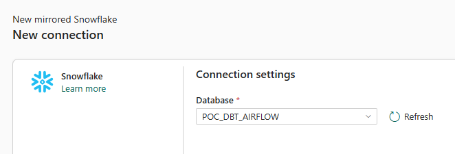
Figure 8: Choose Database

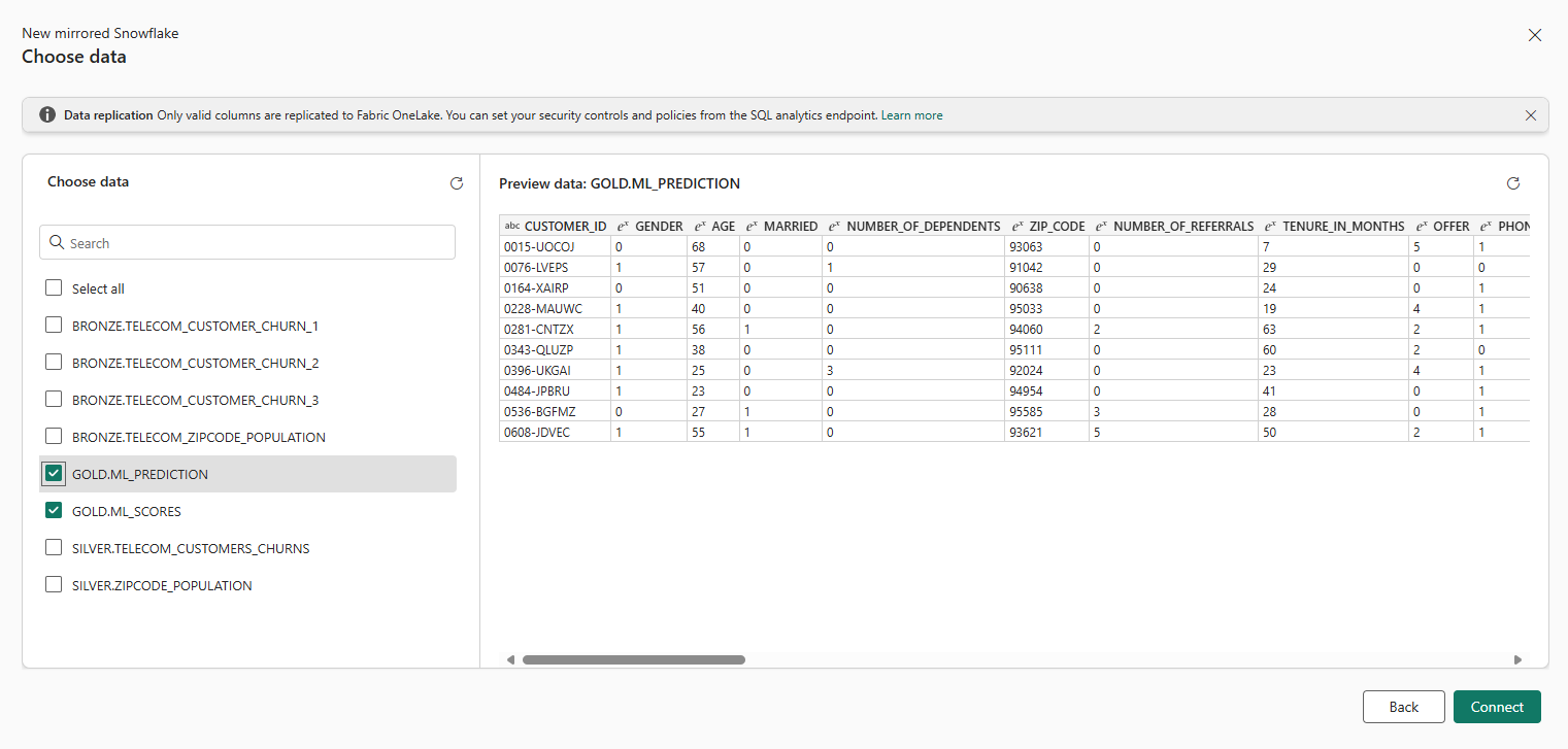
Figure 9: Choose Table

This may take a while, depending on the amount of data we want to move, but once completed, the semantic model and SQL analytics endpoint will appear in our workspace, ready for use:

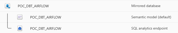
Figure 10: Mirrored Database in the Workspace

If we go into the SQL endpoint, we can see the imported tables and start working with them, executing SQL queries, creating views, and exporting data to Excel if necessary. This serves as a final verification step to ensure we have the latest data available before beginning our analysis:

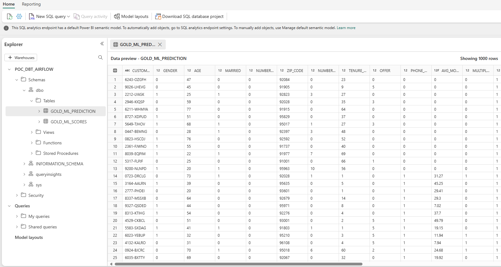
Figure 11: SQL Endpoint

Before finalising and viewing the report in Power BI, we can click on the mirrored database to monitor the replication process, and check the amount of data replicated, track replication times, and identify any failures in any of the tables. At the moment, these monitoring features are fairly basic:

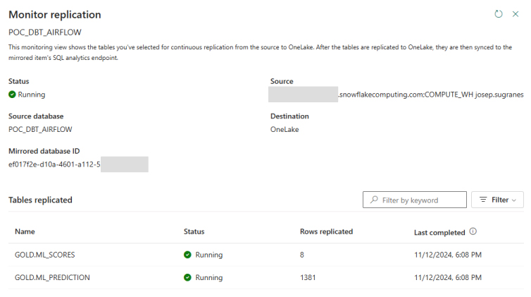
Figure 12: Monitor Replication

At last, it’s time to connect to Power BI and visualise the data we have transformed, using our trained model to predict whether a user is likely to leave the company. To do this, we’ll select the dataset or semantic model, and then click on Create Report:

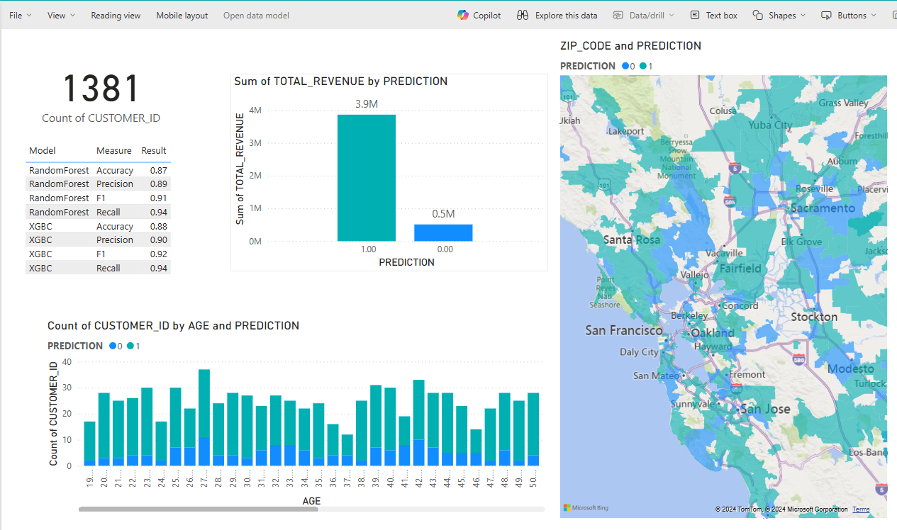
Figure 13: Power BI report

Conclusion

In this second article on data orchestration in Airflow, with Snowflake as a data warehouse, we’ve demonstrated how to create a comprehensive, end-to-end data pipeline. Our solution combines Azure Blob Storage, Snowflake, dbt, Airflow, Snowpark, and Microsoft Fabric into an efficient, fully integrated system. Azure provides secure staging for raw data, which is transformed in Snowflake using dbt. Airflow orchestrates each step, automating the tasks to ensure timely, reliable updates.

Machine learning is handled within Snowflake via Snowpark, allowing models like XGBoost and Random Forest to be trained and evaluated directly on the data. Data is then mirrored to Microsoft Fabric, providing easy access for reporting and visualisation in Power BI. This setup, from ingestion to visualisation, not only optimises data governance, scalability, and accessibility, but also enables centralised predictive analytics and reporting.

Do you have any questions about this blog post, or need some expert guidance on your data transformation journey? Whether you’re looking to simplify your projects, integrate advanced functionalities, or to explore tools like Airflow, Snowflake, Microsoft Fabric and more, our team of experts is here to help, so get in touch today!